Tutorial on the Visualization of Results
Data visualization is a critical aspect of analyzing and interpreting simulation results. In this notebook, you’ll learn how to leverage QuantumDNA’s predefined plotting routines to effectively visualize the outcomes of your calculations.
Examples Covered:
Visualizing the Eigenspectrum Gain insights into the electronic structure by plotting the eigenspectrum of your system. This visualization highlights energy levels and their distributions, essential for analyzing the quantum states of your model.
Visualizing the Fourier Analysis Explore frequency-domain characteristics using Fourier analysis. This technique is particularly useful for identifying periodicities and resonances in quantum systems.
Visualizing Coherences and Populations Delve into the dynamics of quantum states by visualizing coherences and populations of the DNA bases or basepairs. These plots reveal how quantum superpositions evolve over time, providing a window into processes such as energy transfer, decoherence, and relaxation.
By the end of this notebook, you’ll have a grasp of how to utilize qDNA’s visualization capabilities to analyze and communicate your results effectively.
![]()
[1]:
%load_ext autoreload
%autoreload 2

# Save flag: Set to True to enable saving results (currently unused in this script)
save = False

# Verbose flag: Set to True to enable detailed logging
verbose = False
Setup
[2]:
import numpy as np
import matplotlib.pyplot as plt

# --------------------------
# Installation of QuantumDNA
# --------------------------

from importlib.util import find_spec

qDNA_installed = find_spec('qDNA') is not None

if not qDNA_installed:
    %pip install qDNA
    print("Successfully installed the 'qDNA' package.")
else:
    print("Package 'qDNA' is already installed.")

if verbose:
    %pip show qDNA

from qDNA import *

# ------------------------
# Directory Setup
# ------------------------

import os

# Use the current working directory as the root
ROOT_DIR = os.getcwd()

# Define directory to save figures
SAVE_DIR = os.path.join(DATA_DIR, "my_figures")
os.makedirs(SAVE_DIR, exist_ok=True)

if verbose:
    print(f"Save directory: '{SAVE_DIR}' is ready.")
Package 'qDNA' is already installed.
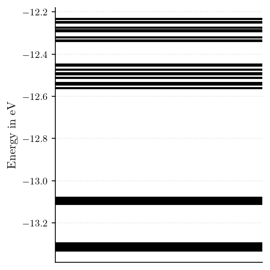
Visualization of the Eigenspectrum
[4]:
tb_sites = get_tb_sites('GCG')
vis = Visualization(tb_sites, tb_model_name='ELM')
fig, ax = vis.plot_eigv()
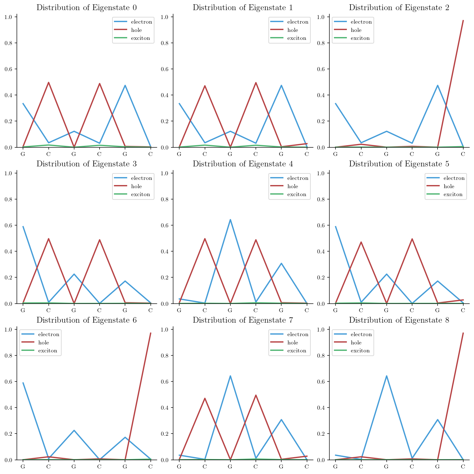
[6]:
tb_sites = get_tb_sites('GCG')
vis = Visualization(tb_sites, tb_model_name='ELM')

num_rows, num_cols = 3, 3
fig, axes = plt.subplots(num_rows, num_cols, figsize=(3.4*num_cols, 3.4*num_rows) )
for i, ax in enumerate(axes.flatten()[:num_rows*num_cols]):
    vis.plot_eigs(i, ax=ax, fig=fig)
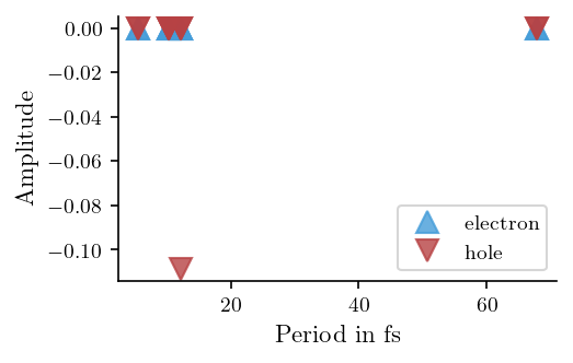
Fourier Analysis
[17]:
tb_sites = get_tb_sites('GA')
vis = Visualization(tb_sites, particles=['electron', 'hole'], tb_model_name = 'WM')
tb_site = '(0, 1)'
fig, ax = vis.plot_fourier( vis.init_states[0], tb_site, 'period')
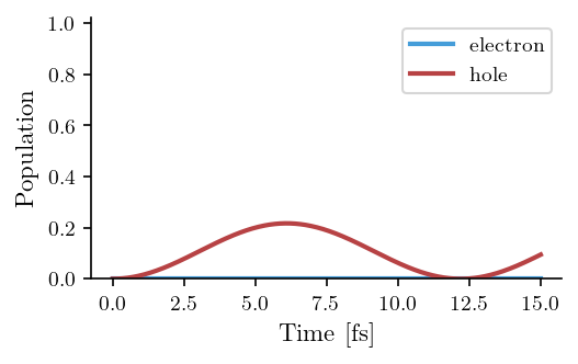
[16]:
tb_sites = get_tb_sites('GA')
vis = Visualization(tb_sites, particles=['electron', 'hole'], tb_model_name = 'WM', t_end=15, t_unit='fs')
tb_site = '(0, 1)'
fig, ax = vis.plot_pop_fourier(vis.init_states[0], tb_site, vis.times, vis.t_unit)
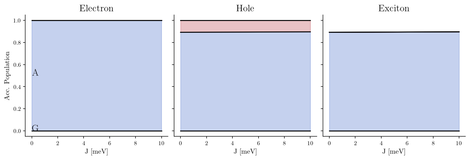
[23]:
tb_sites = get_tb_sites('GA', tb_model_name='WM')
vis = Visualization(tb_sites, tb_model_name = 'WM')
J_list, J_unit = np.linspace(0,10,100), 'meV'

vis.plot_average_pop(J_list, J_unit=J_unit)
Visualization of Populations and Coherences
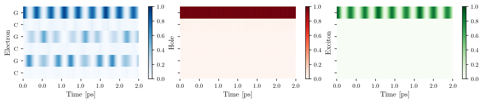
[25]:
tb_sites = get_tb_sites('GCG')
vis = Visualization(tb_sites, source="Hawke2010", t_end=2)
fig, ax = vis.plot_heatmap()
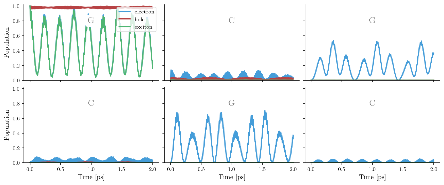
[26]:
tb_sites = get_tb_sites('GCG')
vis = Visualization(tb_sites, source="Hawke2010", t_end=2)
fig, ax = vis.plot_pops()
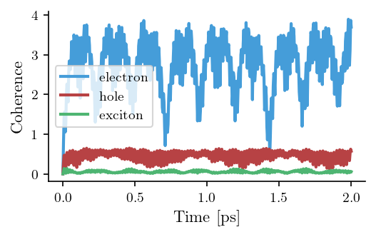
[27]:
tb_sites = get_tb_sites('GCG')
vis = Visualization(tb_sites, source="Hawke2010", t_end=2)
fig, ax = vis.plot_coh()
[ ]: