Tutorial on the Simulation of the DNA Environment
Discover how to model DNA excited-state relaxation and environmental interactions using dephasing and thermalization models from Quantum Biology. This notebook explores various methods for incorporating DNA environment effects and exciton relaxation in the qDNA package. Key topics include:
Local & Global Dephasing: Analyzing the impact of environmental noise on quantum states.
Local & Global Thermalizing: Modeling the system’s approach to thermal equilibrium.
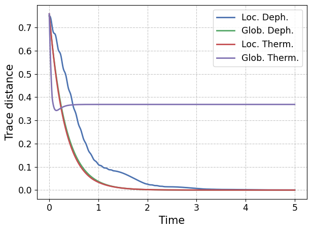
Trace Distance to Equilibrium: Measuring how close the system is to its equilibrium state.
Through these examples, the notebook demonstrates techniques for simulating and analyzing DNA-related quantum phenomena in the presence of an environment.
![]()
[3]:
%load_ext autoreload
%autoreload 2

# Save flag: Set to True to enable saving results (currently unused in this script)
save = False

# Verbose flag: Set to True to enable detailed logging
verbose = False
Setup
[4]:
import numpy as np
import matplotlib.pyplot as plt

# --------------------------
# Installation of QuantumDNA
# --------------------------

from importlib.util import find_spec

qDNA_installed = find_spec('qDNA') is not None

if not qDNA_installed:
    %pip install qDNA
    print("Successfully installed the 'qDNA' package.")
else:
    print("Package 'qDNA' is already installed.")

if verbose:
    %pip show qDNA

# ------------------------
# Directory Setup
# ------------------------

import os

# Use the current working directory as the root
ROOT_DIR = os.getcwd()

# Define directory to save figures
SAVE_DIR = os.path.join(ROOT_DIR, "my_figures")
os.makedirs(SAVE_DIR, exist_ok=True)

if verbose:
    print(f"Save directory: '{SAVE_DIR}' is ready.")
Package 'qDNA' is already installed.
Function Definitions
[5]:
from qDNA import get_deph_eq_state, get_therm_eq_state, get_pop_particle, plot_pop, plot_coh, get_reduced_dm

def my_plot_pop(me_solver):
    if me_solver.lindblad_diss.loc_deph_rate:
        lindblad_type = "local dephasing"
    elif me_solver.lindblad_diss.glob_deph_rate:
        lindblad_type = "global dephasing"
    elif me_solver.lindblad_diss.loc_therm:
        lindblad_type = "local thermalizing"
    elif me_solver.lindblad_diss.glob_therm:
        lindblad_type = "global thermalizing"

    if lindblad_type in ["local dephasing", "global dephasing"]:
        eq_state = get_deph_eq_state(me_solver)
    if lindblad_type in ["local thermalizing", "global thermalizing"]:
        eq_state = get_therm_eq_state(me_solver)

    print(f"Number of {lindblad_type} operators: {me_solver.lindblad_diss.num_c_ops}")
    print("--------------------------------")

    pop_particle_dict = {}
    for particle in me_solver.tb_ham.particles:
        pop_particle_op = get_pop_particle(me_solver.tb_ham.tb_basis, particle, tb_site)
        pop_particle = np.trace(eq_state @ pop_particle_op)
        pop_particle_dict[particle] = pop_particle
        print(f"Equilibium Population {particle.capitalize()}: {round(pop_particle, 3)}")

    fig, ax = plt.subplots()
    plot_pop(ax, tb_site, me_solver)
    for particle in me_solver.tb_ham.particles:
        ax.axhline(y=pop_particle_dict[particle], color='k', linestyle='--', alpha=0.5)

    return fig, ax

def my_plot_coh(me_solver):
    if me_solver.lindblad_diss.loc_deph_rate:
        lindblad_type = "local dephasing"
    elif me_solver.lindblad_diss.glob_deph_rate:
        lindblad_type = "global dephasing"
    elif me_solver.lindblad_diss.loc_therm:
        lindblad_type = "local thermalizing"
    elif me_solver.lindblad_diss.glob_therm:
        lindblad_type = "global thermalizing"

    if lindblad_type in ["local dephasing", "global dephasing"]:
        eq_state = get_deph_eq_state(me_solver)
    if lindblad_type in ["local thermalizing", "global thermalizing"]:
        eq_state = get_therm_eq_state(me_solver)

    print(f"Number of local dephasing operators: {me_solver.lindblad_diss.num_c_ops}")
    print("--------------------------------")

    coh_particle_dict = {}
    for particle in me_solver.tb_ham.particles:
        reduced_dm = get_reduced_dm(eq_state, particle, me_solver.tb_ham.tb_basis)
        coh_particle = np.sum(np.abs(reduced_dm)).real - np.sum(np.diag(reduced_dm)).real
        coh_particle_dict[particle] = coh_particle
        print(f"Equilibium Coherence {particle.capitalize()}: {round(coh_particle, 3)}")

    fig, ax = plt.subplots()
    plot_coh(ax, me_solver)
    for particle in me_solver.tb_ham.particles:
        ax.axhline(y=coh_particle_dict[particle], color='k', linestyle='--', alpha=0.5)

    return fig, ax
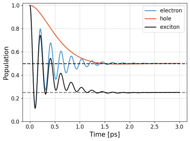
Local Dephasing
[7]:
from qDNA import get_me_solver, save_figure

kwargs = dict(description='2P', loc_deph_rate=5)
upper_strand, tb_model_name = 'GC', 'WM'
tb_site = '(0, 0)'

me_solver = get_me_solver(upper_strand, tb_model_name, **kwargs)
fig, ax = my_plot_pop(me_solver)

if save:
    fig_filename = input("Filename for Saving: ")
    plt.savefig(os.path.join(SAVE_DIR, fig_filename + '.pdf'))
Number of local dephasing operators: 4
--------------------------------
Equilibium Population Electron: 0.5
Equilibium Population Hole: 0.5
Equilibium Population Exciton: 0.25
[8]:
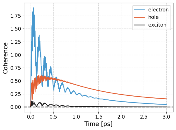
# since the equilibrium state does not contain off-diagonal elements the coherence relaxes to zero

from qDNA import get_me_solver, save_figure

kwargs=dict(description='2P', loc_deph_rate=5)
upper_strand, tb_model_name= 'GC', 'ELM'

me_solver = get_me_solver(upper_strand, tb_model_name, **kwargs)
fig, ax = my_plot_coh(me_solver)

if save:
    fig_filename = input("Filename for Saving: ")
    plt.savefig(os.path.join(SAVE_DIR, fig_filename + '.pdf'))
Number of local dephasing operators: 8
--------------------------------
Equilibium Coherence Electron: 0.0
Equilibium Coherence Hole: 0.0
Equilibium Coherence Exciton: 0.0
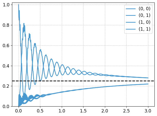
[9]:
from qDNA import get_me_solver, plot_pop, get_deph_eq_state, get_pop_particle

kwargs = dict(description='2P', particles=['electron'], loc_deph_rate=4)
upper_strand, tb_model_name = 'GC', 'ELM'

me_solver = get_me_solver(upper_strand, tb_model_name, **kwargs)
eq_state = get_deph_eq_state(me_solver)
tb_basis = me_solver.tb_ham.tb_basis
particle = me_solver.tb_ham.particles[0]

pop_particle_dict = {}
for tb_site in tb_basis:
    pop_particle_op = get_pop_particle(tb_basis, particle, tb_site)
    pop_particle = np.trace(eq_state @ pop_particle_op)
    pop_particle_dict[tb_site] = pop_particle
    print(f"Equilibium Population {particle.capitalize()} at site {tb_site}: {round(pop_particle, 3)}")

fig, ax = plt.subplots()
for tb_site in tb_basis:
    plot_pop(ax, tb_site, me_solver, add_legend=False)
ax.legend(tb_basis)
for tb_site in tb_basis:
    ax.axhline(y=pop_particle_dict[tb_site], color='k', linestyle='--', alpha=0.5)

if save:
    fig_filename = input("Filename for Saving: ")
    plt.savefig(os.path.join(SAVE_DIR, fig_filename + '.pdf'))
Equilibium Population Electron at site (0, 0): 0.25
Equilibium Population Electron at site (0, 1): 0.25
Equilibium Population Electron at site (1, 0): 0.25
Equilibium Population Electron at site (1, 1): 0.25
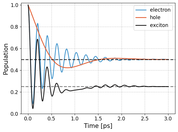
Global Dephasing
[10]:
from qDNA import get_me_solver, save_figure

kwargs = dict(description='2P', glob_deph_rate=2)
upper_strand, tb_model_name = 'GC', 'WM'
tb_site = '(0, 0)'

me_solver = get_me_solver(upper_strand, tb_model_name, **kwargs)
fig, ax = my_plot_pop(me_solver)

if save:
    fig_filename = input("Filename for Saving: ")
    plt.savefig(os.path.join(SAVE_DIR, fig_filename + '.pdf'))
Number of global dephasing operators: 4
--------------------------------
Equilibium Population Electron: 0.5
Equilibium Population Hole: 0.5
Equilibium Population Exciton: 0.25
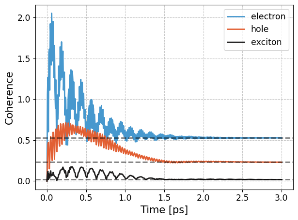
[11]:
# the equilibirum state contains off-diagonal elements indicating the coherences even in the equilibrium.

from qDNA import get_me_solver, save_figure

kwargs=dict(description='2P', glob_deph_rate=2)
upper_strand, tb_model_name= 'GC', 'ELM'

me_solver = get_me_solver(upper_strand, tb_model_name, **kwargs)
fig, ax = my_plot_coh(me_solver)

if save:
    fig_filename = input("Filename for Saving: ")
    plt.savefig(os.path.join(SAVE_DIR, fig_filename + '.pdf'))
Number of local dephasing operators: 16
--------------------------------
Equilibium Coherence Electron: 0.527
Equilibium Coherence Hole: 0.23
Equilibium Coherence Exciton: 0.017
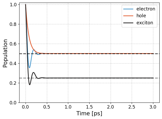
Local Thermalizing
[11]:
from qDNA import get_me_solver, save_figure

kwargs = dict(description='2P', loc_therm=True)
upper_strand, tb_model_name = 'GC', 'WM'
tb_site = '(0, 0)'

me_solver = get_me_solver(upper_strand, tb_model_name, **kwargs)
fig, ax = my_plot_pop(me_solver)

if save:
    fig_filename = input("Filename for Saving: ")
    plt.savefig(os.path.join(SAVE_DIR, fig_filename + '.pdf'))
Number of local thermalizing operators: 52
--------------------------------
Equilibium Population Electron: 0.5
Equilibium Population Hole: 0.5
Equilibium Population Exciton: 0.25
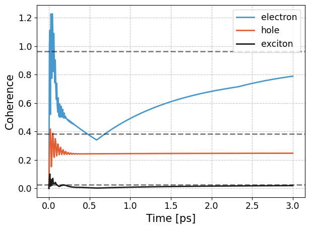
[12]:
from qDNA import get_me_solver, save_figure

kwargs=dict(description='2P', loc_therm=True)
upper_strand, tb_model_name= 'GC', 'ELM'

me_solver = get_me_solver(upper_strand, tb_model_name, **kwargs)
fig, ax = my_plot_coh(me_solver)

if save:
    fig_filename = input("Filename for Saving: ")
    plt.savefig(os.path.join(SAVE_DIR, fig_filename + '.pdf'))
Number of local dephasing operators: 3728
--------------------------------
Equilibium Coherence Electron: 0.963
Equilibium Coherence Hole: 0.384
Equilibium Coherence Exciton: 0.027
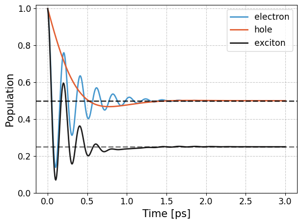
Global Thermalizing
[13]:
from qDNA import get_me_solver, save_figure

kwargs = dict(description='2P', glob_therm=True)
upper_strand, tb_model_name = 'GC', 'WM'
tb_site = '(0, 0)'

me_solver = get_me_solver(upper_strand, tb_model_name, **kwargs)
fig, ax = my_plot_pop(me_solver)

if save:
    fig_filename = input("Filename for Saving: ")
    plt.savefig(os.path.join(SAVE_DIR, fig_filename + '.pdf'))
Number of global thermalizing operators: 12
--------------------------------
Equilibium Population Electron: 0.5
Equilibium Population Hole: 0.5
Equilibium Population Exciton: 0.25
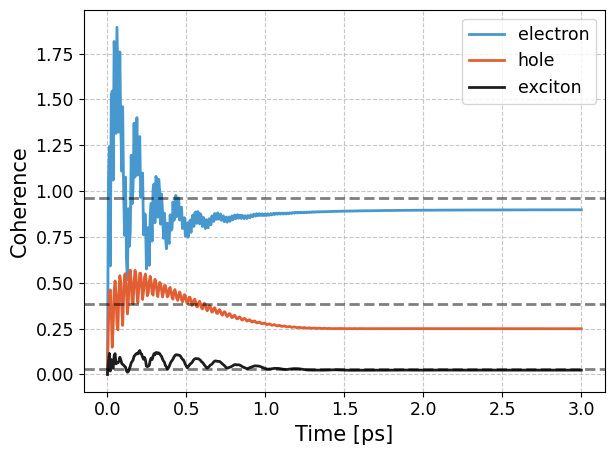
[14]:
from qDNA import get_me_solver, save_figure

kwargs=dict(description='2P', glob_therm=True)
upper_strand, tb_model_name= 'GC', 'ELM'

me_solver = get_me_solver(upper_strand, tb_model_name, **kwargs)
fig, ax = my_plot_coh(me_solver)

if save:
    fig_filename = input("Filename for Saving: ")
    plt.savefig(os.path.join(SAVE_DIR, fig_filename + '.pdf'))
Number of local dephasing operators: 240
--------------------------------
Equilibium Coherence Electron: 0.963
Equilibium Coherence Hole: 0.384
Equilibium Coherence Exciton: 0.027
Trace Distance to the Equilibium
[12]:
from qDNA import calc_trace_distance

upper_strand, tb_model_name= 'GC', 'WM'

kwargs_loc_deph = dict(description='2P', loc_deph_rate=3, relaxation=False, t_end=5)
kwargs_glob_deph = dict(description='2P', glob_deph_rate=3, relaxation=False, t_end=5)
kwargs_loc_therm = dict(description='2P', loc_therm=True, relaxation=False, t_end=5)
kwargs_glob_therm = dict(description='2P', glob_therm=True, relaxation=False, t_end=5)
kwargs_list = [kwargs_loc_deph, kwargs_glob_deph, kwargs_loc_therm, kwargs_glob_therm]

trace_distance_list = []
for kwargs in kwargs_list:
    me_solver = get_me_solver(upper_strand, tb_model_name, **kwargs)
    if me_solver.lindblad_diss.loc_deph_rate or me_solver.lindblad_diss.glob_deph_rate:
        eq_state = get_deph_eq_state(me_solver)
    if me_solver.lindblad_diss.loc_therm or me_solver.lindblad_diss.glob_therm:
        eq_state = get_therm_eq_state(me_solver)
    dms = me_solver.get_result()
    trace_distance = [ calc_trace_distance(dm.full(), eq_state) for dm in dms ]
    trace_distance_list.append(trace_distance)

fig, ax = plt.subplots()
for trace_distance in trace_distance_list:
    ax.plot(me_solver.times, trace_distance)
ax.legend(['Loc. Deph.', 'Glob. Deph.', 'Loc. Therm.', 'Glob. Therm.'])
ax.set_ylabel('Trace distance')
ax.set_xlabel('Time')

if save:
    fig_filename = input("Filename for Saving: ")
    plt.savefig(os.path.join(SAVE_DIR, fig_filename + '.pdf'))